Once you have installed Quartus 11.1 sp2 Web Edition and ModelSim 10.0c Altera Starter Edition from the Software Downloads page, this tutorial will help you use those two programs to write, compile, and execute your projects.
NOTE: You should install Quartus first and then ModelSim.
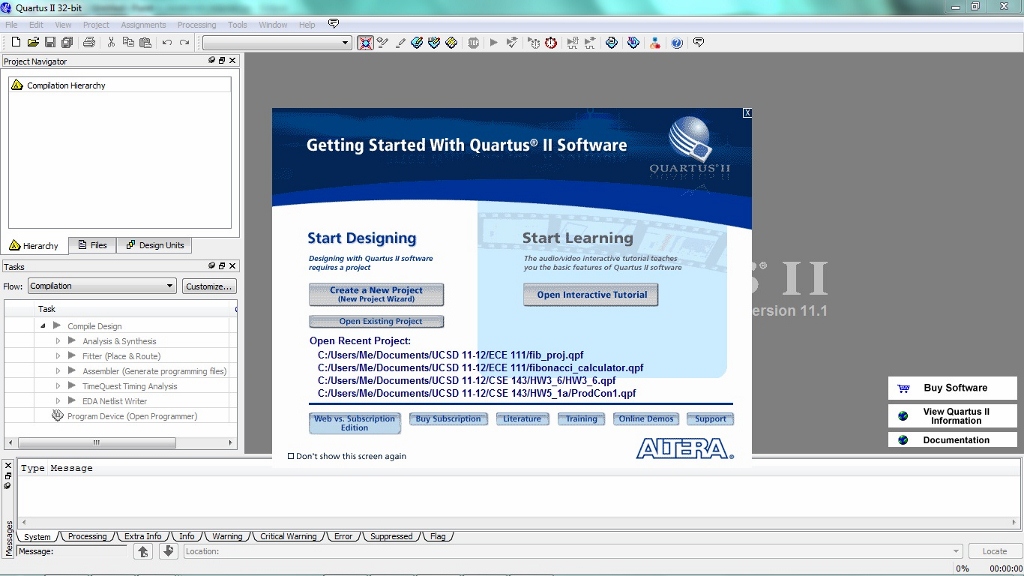
We start off by running Quartus. You will be greeted by the following welcome screen. If you are starting a new project, click on Create a New Project. If you are resuming a project, click on Open Existing Project.
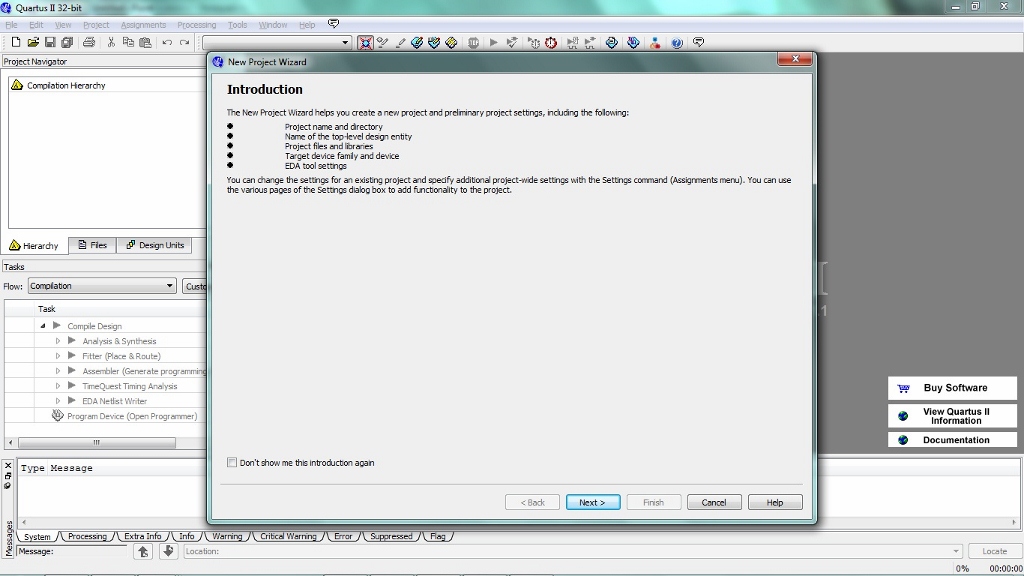
The Introduction Page will show up. Simply press Next.
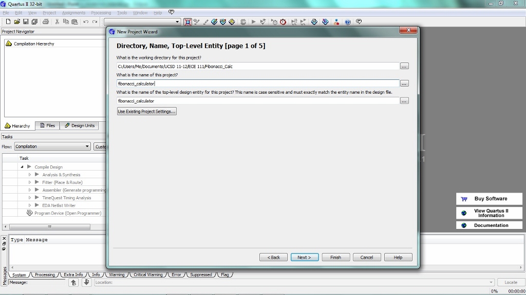
You will be asked to select a working directory for the project. Select a directory where you want your project to be saved. Be aware that you cannot have multiple projects in the same directory. If you have a directory for this class, there should be sub-folders for each project. The name of the project has to match the name of one of the files in the project. In this screenshot, the project name is fobonacci_calculator because there will be a fibonacci_calculator.v file in the project. Once this is complete, select Next.
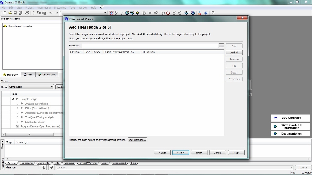
The next screen allows you to add files to the project is already created on your computer. After you have selected the files to add (if any), press Next.
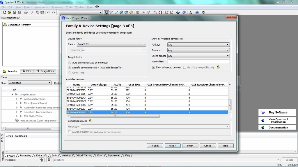
Designing hardware relies on the capability of each FPGA. In this class, we will be using:
Family: Arria II GX
Device: EP2AGX45DF29I5
This is the last device on the list. Be sure to use this device otherwise your area and timing numbers will be incorrect. Press Next.
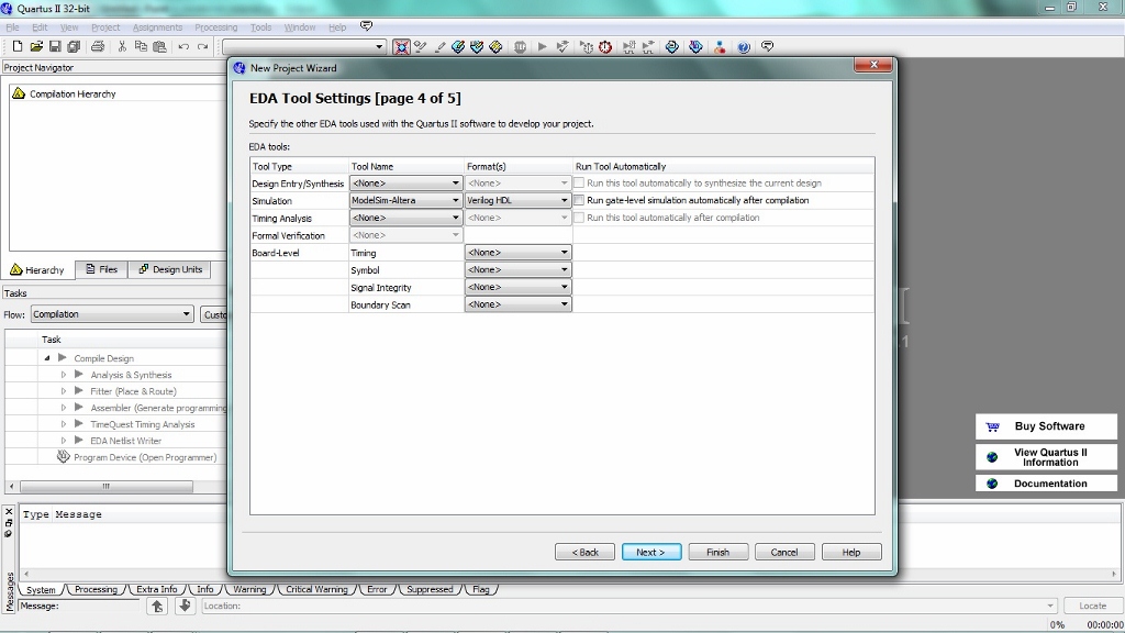
The next page asks to specify which tools you will be using. The simulation Tool Name should be ModelSim-Altera and Format is Verilog HDL. Press Next.
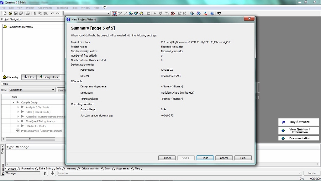
On the Summary page, press Finish.
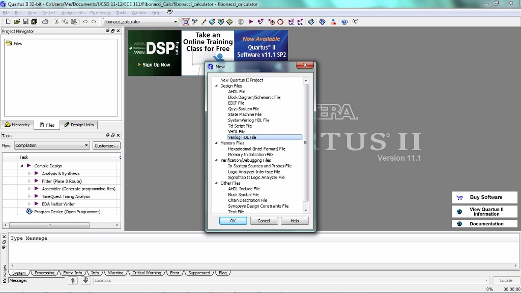
Now that you have created your project, you can start coding. Go to File-->New. Select Verilog HDL File.
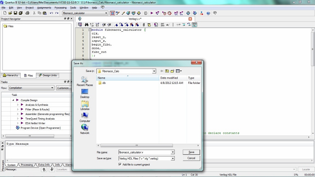
Once a new file is created, you are able to enter your code into it. When you save it, you have to have the module name and file name match up. Remember that one of the file names must match the name of the project. Double check the Save as type is Verilog HDL Files.
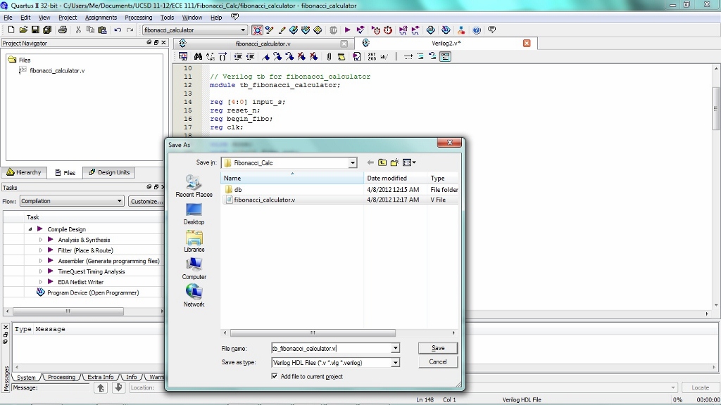
Every project in hardware needs a testbench to generate all necessary inputs and read outputs to ensure they are correct. This is very similar to writing test cases in software programming. The standard way of naming a testbench is to add a "tb_" in front of the name of the module you are testing. In this case, we are testing "fibonacci_calculator" so the name of the new Verilog HDL File is "tb_fibonacci_calculator". A testbench is just a standard Verilog HDL File.
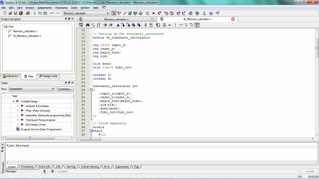
You can see all the project files by clicking on Files on the Project Navigation pane on the left.
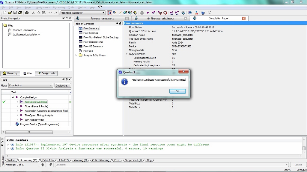
After you have finished coding up your modules, double click on Analysis & Synthesis under the Tasks pane. If you do not see Analysis & Synthesis, double check that Flow is set to Compilation. This will compile and synthesize your program(s). If there are no errors, you will see a pop-up saying the Analysis & Compilation was successful. If not, it will tell you your errors in the Messages pane at the bottom of the screen. It is good habit to just review your warnings (if any) to ensure you have no latches or other design hazards.
Once the Analysis & Synthesis is successful, you can do a RTL Simulation. Go to Tools-->Run Simulation Tool-->RTL Simulation. Another way is to press the icon near the top that is shown boxed below.
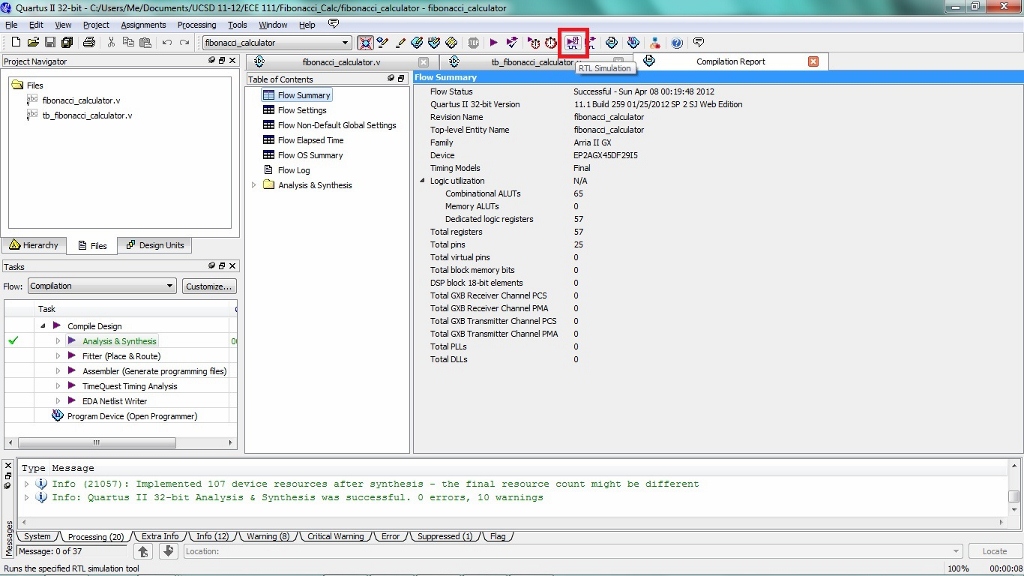
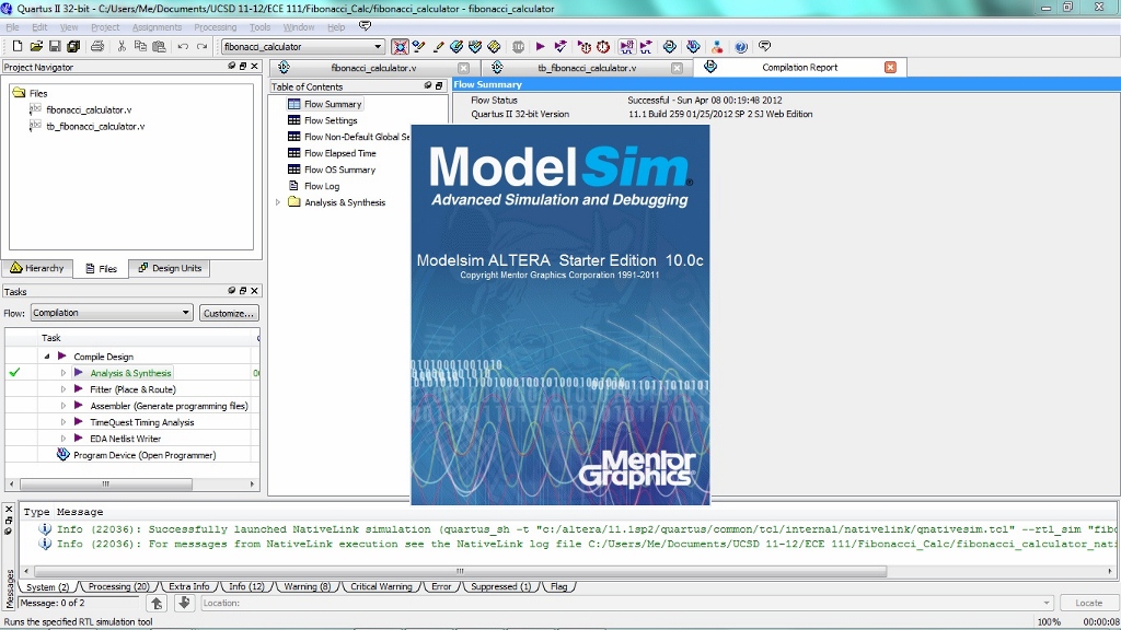
This will launch ModelSim.
The Library you will be working in is called work. Do not bother creating another library as it will cause complications when you try to simulate your program again after closing ModelSim. Expanding the work library will show at least one of the files in your project.
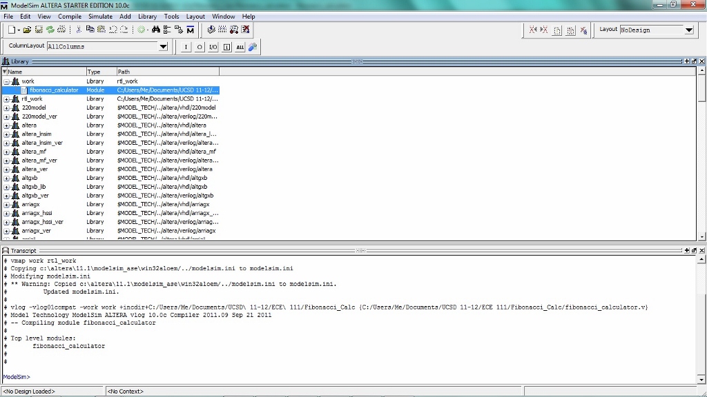
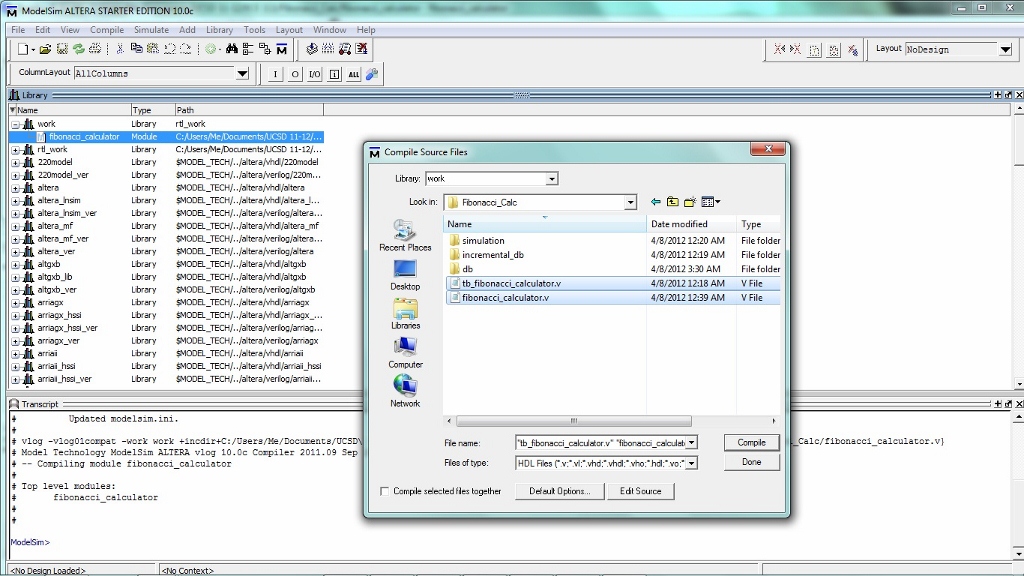
Go to Compile-->Compile. Ensure that the Library is work and you are in your project's directory. Many times you will have to change directories so that you are in your project's directory. Select all Verilog HDL Files that pertain to your project. This includes the testbench. Hit Compile and then Done.
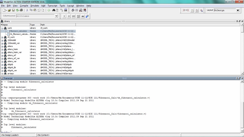
If you look at the bottom in the Transcript pane, you will see that it did compile and there were no errors. The work library should have all the files you just compiled. If not, repeat the previous step. Since the testbench does the signal generations and testing, double click on your testbench file.
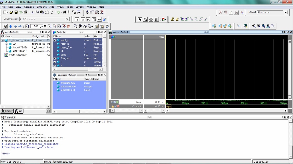
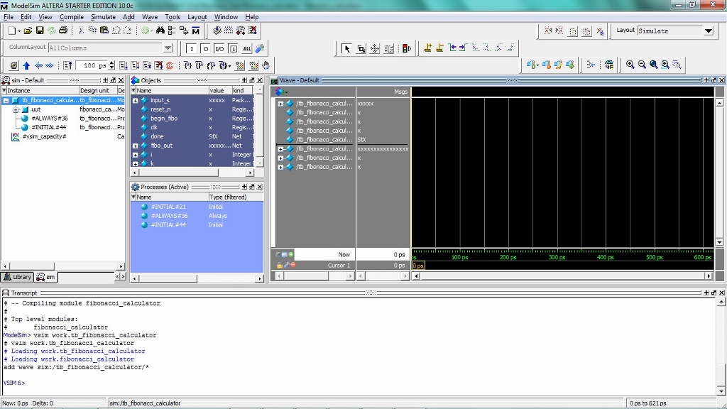
ModelSim will slowly load new panes to look like below. If you do not see the Wave pane, do not worry as you will show it in later steps. You should see something similar to below.
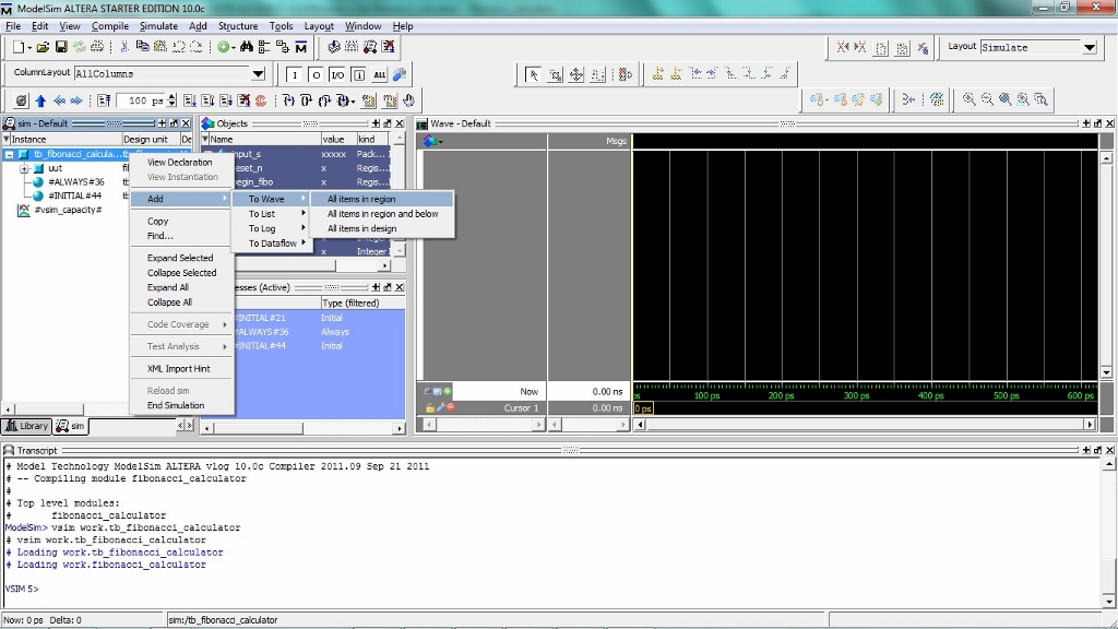
The next step is to add signals to the wave and show the wave if it is not already present. On the left, in the sim pane, right click on the testbench file which should be the top most file. Go to Add-->To Wave-->All items in region.
In the Wave pane, you will see all the signals declared and used in the testbench.
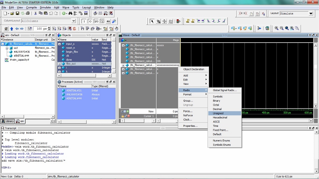
When dealing with signals that are many bits, it is easier to see its value as an unsigned integer rather than binary. To make this conversion, right click on the signal you want, go to Radix and choose the format you want. Unsigned integer is the radix you will use for this class.
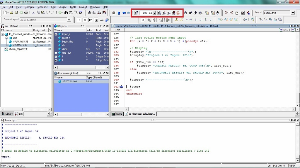
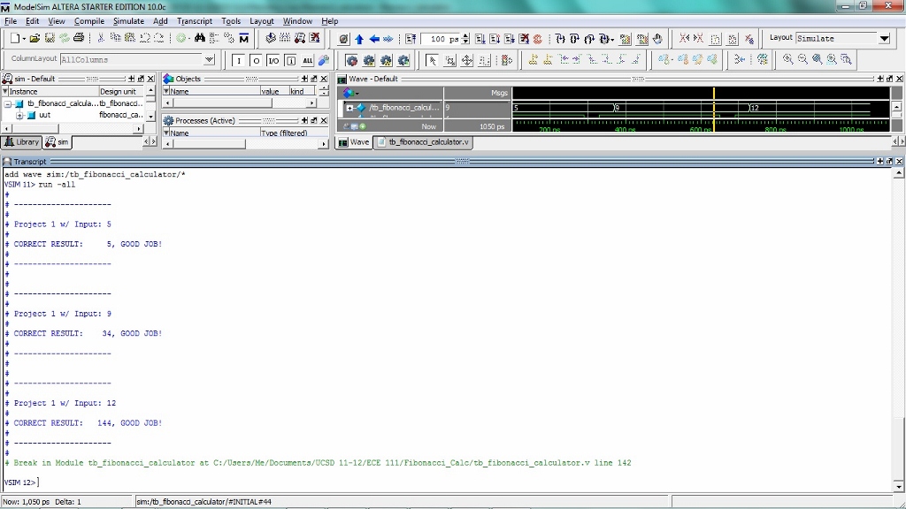
You are now ready to simulate your program. The icons boxed in the below screenshot are used to run the testbench. The first icon is Restart which will reset the simulation as if you never ran it. This is helpful to rerun the simulation without recompiling everything. The Run Length allows you to enter a specific amount of time you want the program to run for. It defaults to pico-seconds, but nano-seconds is the best time to use. The icon Run right after the Run Length is to run your program for the amount of time specified in the Run Length. If you set Run Length to be 10 ns, each time you press Run, the program will continue for 10 ns. Continue Run will run the program until it terminates. The same is true for Run -All. All the programs in this class will terminate in less than one second. If you find yourself waiting for longer than a few seconds until the program terminates, hit the Stop button and recheck your logic. you will see the following screen once your program terminates. It shows you where the program terminated. To go back to the Wave, click on the Wave tab.
You should see something like this on your Wave.
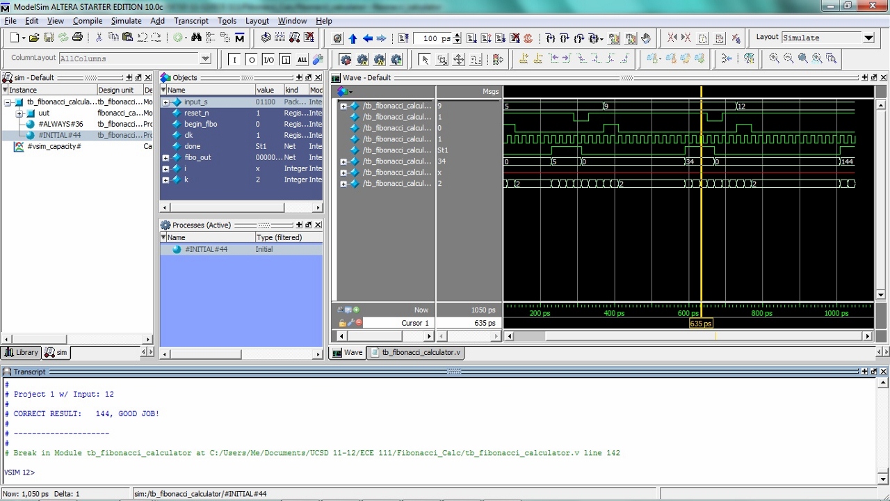
If you expand or scroll through the Transcript pane, you will see the output of any $display statements you have in your code.
To find the area and timing of your program, go back to Quartus and double click on TimeQuest Timing Analysis in the Tasks pane. This will run Fitter (Place & Route) as well. You will get another successful message.
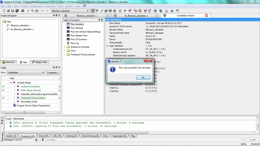
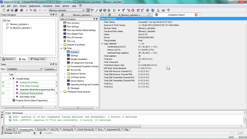
To find area, select the Compilation Report tab and click on Fitter. On the Summary page, you can find the area by adding up the three items under Logic Utilization.
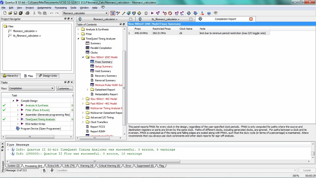
To find the clock frequency, select the Compilation Report tab and click on TimeQuest Timing Analyzer. Click on Slow 900mV 100C Model and look at Fmax Summary. The speed of your clock is given by Fmax.